show code
# Load libraries
library(terra)
library(sf)
library(tidyverse)
library(here)
library(tmap)
library(testthat)As global demand for sustainable protein grows, marine aquaculture offers an alternative to land-based meat production. Gentry et al. found through mapping potential for marine aquaculture using multiple constraints, that global seafood demand could be met using less than 0.015% of global ocean area.
This exercise determines which Exclusive Economic Zones (EEZ) on the West Coast of the US are best suited to developing marine aquaculture to several species of oysters, and develops a function for visualizing suitability based on a single species—Pteria sterna, the Pacific winged oyster—in this case.
# Load libraries
library(terra)
library(sf)
library(tidyverse)
library(here)
library(tmap)
library(testthat)# Source external script that defines a custom function for aquaculture suitability
source(here::here("posts/2024-12-24-aquaculture-suitability/suitable-aquaculture.R"))This function will also be provided below as part of hwk4.qmd.
# Read in Sea Surface Temperature, Bathymetry, and EEZ data
files <- list.files(here::here("posts/2024-12-24-aquaculture-suitability/data"), pattern = "average*", full.names = TRUE)
sst <- terra::rast(files)
names(sst) <- c(2008, 2009, 2010, 2011, 2012)

if (nlyr(sst) == 0) {
  stop("No layers found in SST data")
}

depth <- terra::rast(here::here("posts/2024-12-24-aquaculture-suitability/data", "depth.tif")) %>%
  project(., y = crs(sst))

wc_eez <- st_read(here::here("posts/2024-12-24-aquaculture-suitability/data", "wc_regions_clean.shp"), quiet = TRUE) %>%
st_transform(., crs = crs(sst))# Check that the CRSs match for the datasets
testthat::test_that("Coordinate reference systems match", {
expect_equal(crs(sst), crs(depth))
expect_equal(crs(depth), crs(wc_eez))
})Test passed 🎊# Import US state boundaries for plotting
states <- st_read(here::here("posts/2024-12-24-aquaculture-suitability/data", "states", "cb_2023_us_state_20m.shp"), quiet = TRUE) %>%
filter(NAME %in% c("California", "Oregon", "Washington", "Nevada")) %>%
st_transform(., crs = crs(sst)) %>%
st_crop(., st_bbox(wc_eez))sst_mean <- sst %>%
terra::mean() %>%
- 273.15 # Convert from ºK to ºC
depth_cropped <- crop(depth, sst_mean)
if (res(depth_cropped)[1] != res(sst_mean)[1]) {
warning(sprintf("Resolution mismatch",
res(depth_cropped)[1], res(sst_mean)[1]))
}
depth_resample <- resample(depth_cropped, sst_mean, method = "near")
ext(depth_resample) == ext(sst_mean)[1] TRUE# Check that the depth and SST rasters match in resolution, extent, and position
depth_sst_stack <- c(depth_resample, sst_mean)Research has shown that oysters need the following conditions for optimal growth:
# Define reclassification matrices for depth and SST
rcl_depth <- matrix(c(-Inf, -70, 0,
                      -70, 0, 1,
                      0, Inf, 0),
                    ncol = 3, byrow = TRUE)
rcl_sst <- matrix(c(-Inf, 11, 0,
                    11, 30, 1,
                    30, Inf, 0),
                  ncol = 3, byrow = TRUE)

# Apply the matrices to the depth and SST rasters, making all cells 0 or 1
depth_rcl <- terra::classify(depth_resample, rcl = rcl_depth)
sst_rcl <- terra::classify(sst_mean, rcl = rcl_sst)

# Find locations that satisfy both SST and depth conditions
suitablility <- function(depth_rcl, sst_rcl) {
  depth_rcl*sst_rcl
}
suitable <- lapp(c(depth_rcl, sst_rcl), fun = suitablility)# Set unsuitable locations to NAs
suitable[suitable == 0] <- NA
# Find the total suitable area within each EEZ
eez_area <- terra::cellSize(suitable, mask = T, unit = "km")
suitable_eez_area <- exactextractr::exact_extract(
eez_area, wc_eez,
fun = "sum",
append_cols=c("rgn", "area_km2"),
progress = FALSE)
# Join to original data to obtain geometries for visualization
suitable_eez_join <- left_join(wc_eez, suitable_eez_area)
tm_shape(suitable_eez_join) +
tm_fill(col = "sum",
style = "pretty",
palette = "Blues",
title = "Suitable Area (km\u00b2)") +
tm_text(text = "rgn",
size = 0.7) +
tm_shape(states) +
tm_polygons(col = "#e3d3b8",
border.col = "#402618") +
tm_shape(wc_eez) +
tm_borders(col = "#402618") +
tm_layout(main.title = paste("Suitable Area for Oyster Fisheries \nin West Coast EEZ"),
bg.color = "#e8ebea",
legend.bg.color = "#e3d3b8",
legend.position = c(0.61, 0.85)) +
tm_scale_bar(position = c("left", "bottom")) +
tm_compass(position = c("right", "bottom"),
size = 2)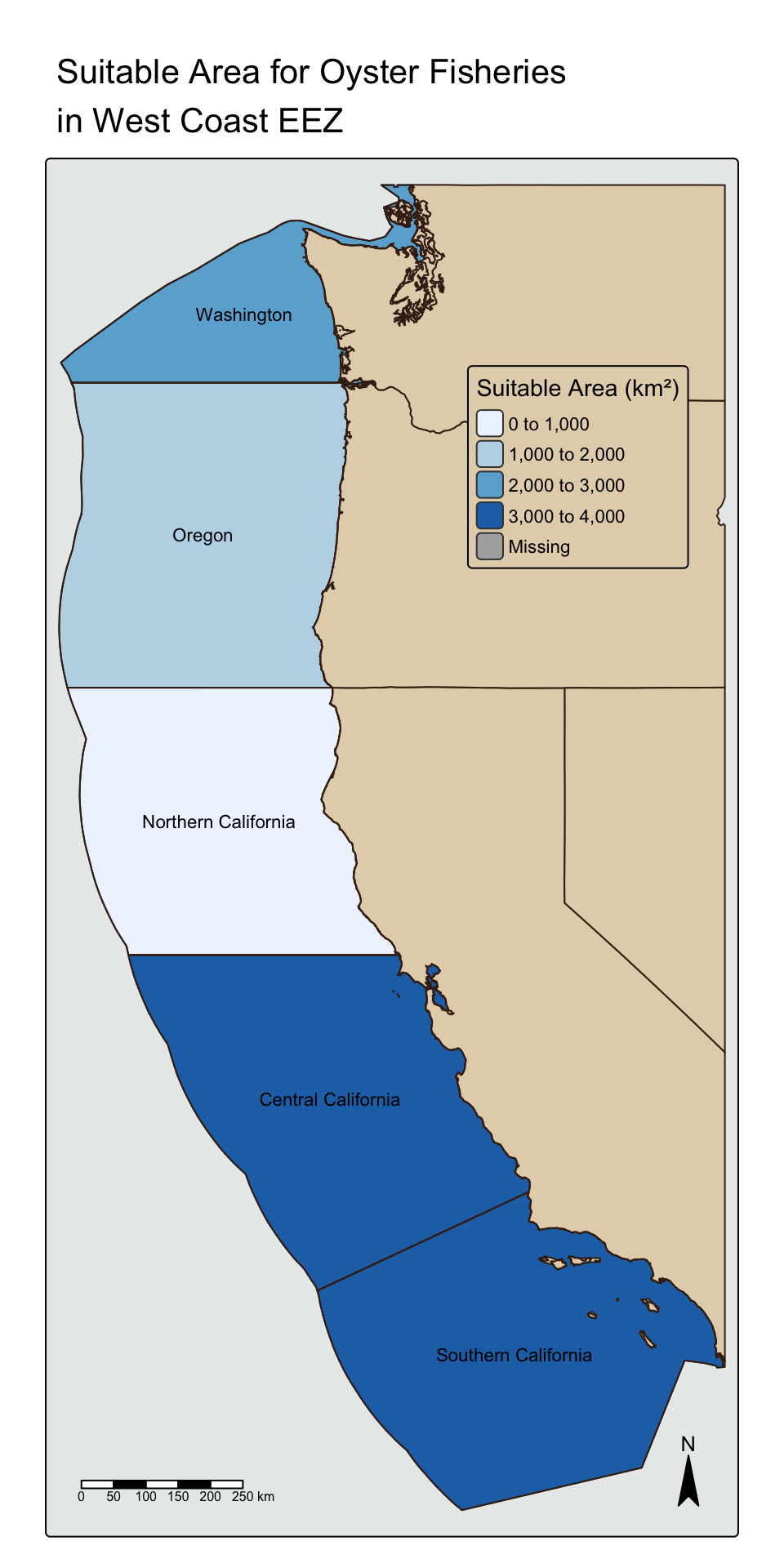
Using the provided depth, sea surface temperature, West Coast Exclusive Economic Zones, and states data, we can conduct a suitability analysis and produce a suitability map for any species of interest for marine aquaculture given their sea surface temperature range, depth range and species name.
suitable_aquaculture <- function(min_temp, max_temp, min_depth, max_depth, species) {
# Read and prepare data
files <- list.files(here::here("posts/2024-12-24-aquaculture-suitability/data"), pattern = "average*", full.names = TRUE)
sst <- terra::rast(files)
names(sst) <- c(2008, 2009, 2010, 2011, 2012)
# Import bathymetry data
depth <- terra::rast(here::here("posts/2024-12-24-aquaculture-suitability/data", "depth.tif"))
# Import EEZ and state boundaries
wc_eez <- st_read(here::here("posts/2024-12-24-aquaculture-suitability/data", "wc_regions_clean.shp"), quiet = TRUE) %>%
st_transform(., crs = crs(sst))
states <- st_read(here::here("posts/2024-12-24-aquaculture-suitability/data", "states", "cb_2023_us_state_20m.shp"), quiet = TRUE) %>%
filter(NAME %in% c("California", "Oregon", "Washington", "Nevada")) %>%
st_transform(., crs = crs(sst)) %>%
st_crop(., st_bbox(wc_eez))
# Process SST data
sst_mean <- sst %>%
terra::mean() %>%
- 273.15 # Convert from Kelvin to Celsius
# Process depth data
depth <- project(depth, y = crs(sst))
depth_cropped <- crop(depth, sst_mean)
depth_resample <- resample(depth_cropped, sst_mean, method = "near")
# Create reclassification matrices
rcl_depth <- matrix(c(-Inf, -max_depth, 0,
-max_depth, min_depth, 1,
min_depth, Inf, 0),
ncol = 3, byrow = TRUE)
rcl_sst <- matrix(c(-Inf, min_temp, 0,
min_temp, max_temp, 1,
max_temp, Inf, 0),
ncol = 3, byrow = TRUE)
# Apply matrices to depth and SST rasters
depth_rcl <- terra::classify(depth_resample, rcl = rcl_depth)
sst_rcl <- terra::classify(sst_mean, rcl = rcl_sst)
# Find locations that satisfy both SST and depth conditions
suitablility <- function(depth_rcl, sst_rcl) {
depth_rcl*sst_rcl
}
suitable <- lapp(c(depth_rcl, sst_rcl), fun = suitablility)
# Set unsuitable locations to NA
suitable[suitable == 0] <- NA
# Find the total suitable area within each EEZ
eez_area <- terra::cellSize(suitable, mask = T, unit = "km")
suitable_eez_area <- exactextractr::exact_extract(eez_area, wc_eez,
fun = "sum",
append_cols=c("rgn", "area_km2"),
progress = FALSE)
# Join to original data to obtain geometries for visualization
suitable_eez_join <- left_join(wc_eez, suitable_eez_area, by = join_by(rgn, area_km2))
# Visualize suitable area
tm_shape(suitable_eez_join) +
tm_fill(col = "sum",
style = "pretty",
palette = "Blues",
title = "Suitable Area (km\u00b2)") +
tm_text(text = "rgn",
size = 0.7) +
tm_shape(states) +
tm_polygons(col = "#e3d3b8",
border.col = "#402618") +
tm_shape(wc_eez) +
tm_borders(col = "#402618") +
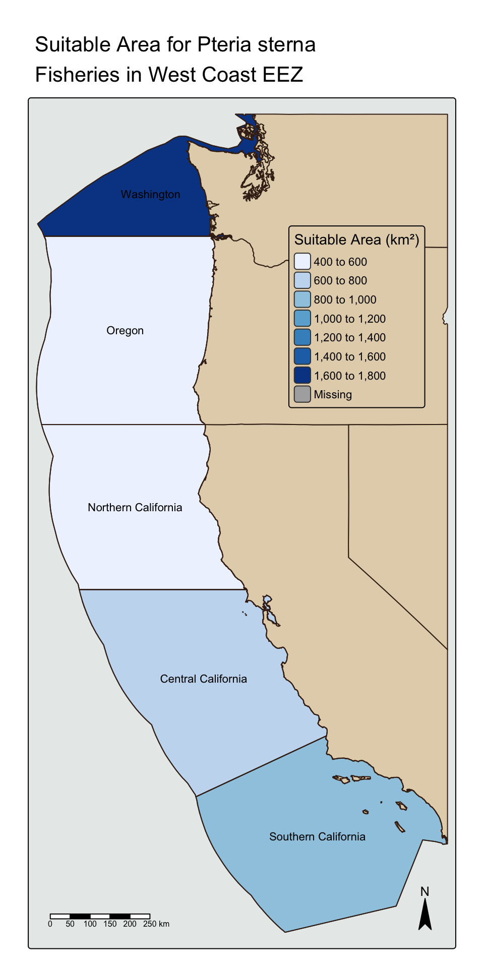
tm_layout(main.title = paste("Suitable Area for",
species,
"\nFisheries in West Coast EEZ"),
bg.color = "#e8ebea",
legend.bg.color = "#e3d3b8",
legend.position = c(0.61, 0.85)) +
tm_scale_bar(position = c("left", "bottom")) +
tm_compass(position = c("right", "bottom"),
size = 2)
}Pteria sterna or the Pacific wing-oyster is an eastern Pacific oyster of commercial value.
Conditions for optimal growth:
suitable_aquaculture(10, 30, 3, 26, "Pteria sterna")
|---------|---------|---------|---------|
=========================================
| Data | Citation | Link |
|---|---|---|
| Sea Surface Temperature | NOAA Coral Reef Watch (2018). NOAA Coral Reef Watch Daily Global 5-km Satellite Sea Surface Temperature Anomaly Product v3.1 | https://coralreefwatch.noaa.gov/product/5km/index_5km_ssta.php |
| Bathymetry | GEBCO Compilation Group (2022) GEBCO_2022 Grid (doi:10.5285/e0f0bb80-ab44-2739-e053-6c86abc0289c) | https://www.gebco.net/data_and_products/gridded_bathymetry_data/#area |
| EEZ Boundaries | Marine Regions - Maritime Boundaries and Exclusive Economic Zones, 2019 | https://www.marineregions.org/eez.php |
| State Boundaries | U.S. Census Bureau TIGER/Line Shapefiles, 2023 | https://www.census.gov/geographies/mapping-files/time-series/geo/tiger-line-file.html |